That’s not my weather station…! Exploring 433MHz

Since I first played around with my first ADC on the BBC Micro in the early ’90s, I’ve always had a bit of a thing for data logging of one sort or another – when building data visualisations or just playing around with datasets it’s usually more fun working with data you’ve collected yourself.

So a few years ago I bought a little weather station to stick up in the garden, mostly for my wife, who’s the gardener, to keep an eye on the temperature, wind, humidity, etc. It has a remote sensor array in the garden running off a few AA batteries and transmitting wirelessly to a base station, with a display, which we keep in the kitchen. The base station also displays indoor temperature & pressure.

I discovered, more recently, that the sensor array transmits its data on 433MHz which is a license-free band for use by low power devices. At around the same time, I also discovered the cheap RTL-SDR repurposed DVB-T USB stick and eventually found my way over to the very convenient rtl_433 project.

Eventually, I wanted to try and build a datalogger for the weather station, but rather than periodically plugging the base station into something to offload the data it already captures, or leave something ugly plugged into the base station in the kitchen, I figured I’d configure a spare raspberry pi with rtl_433 and run it somewhere out of the way, so I duly went ahead and did that. It works really well and I’ve added a basic web UI which mimics the original base station display and combines it with data from elsewhere (like moon phases) and my intention is eventually to combine all sorts of other stuff like APT weather satellite imagery and maybe even sunspot activity for my other radio-based interests.

Even though the capture has been running permanently for at least a year now I’ve never really gone back to look at the data being logged, which was one of my original plans (temperature trend plots). Having a poke around the data this morning reminded me that actually there are lots of other things which broadcast on the same frequency and I wanted to share them here.

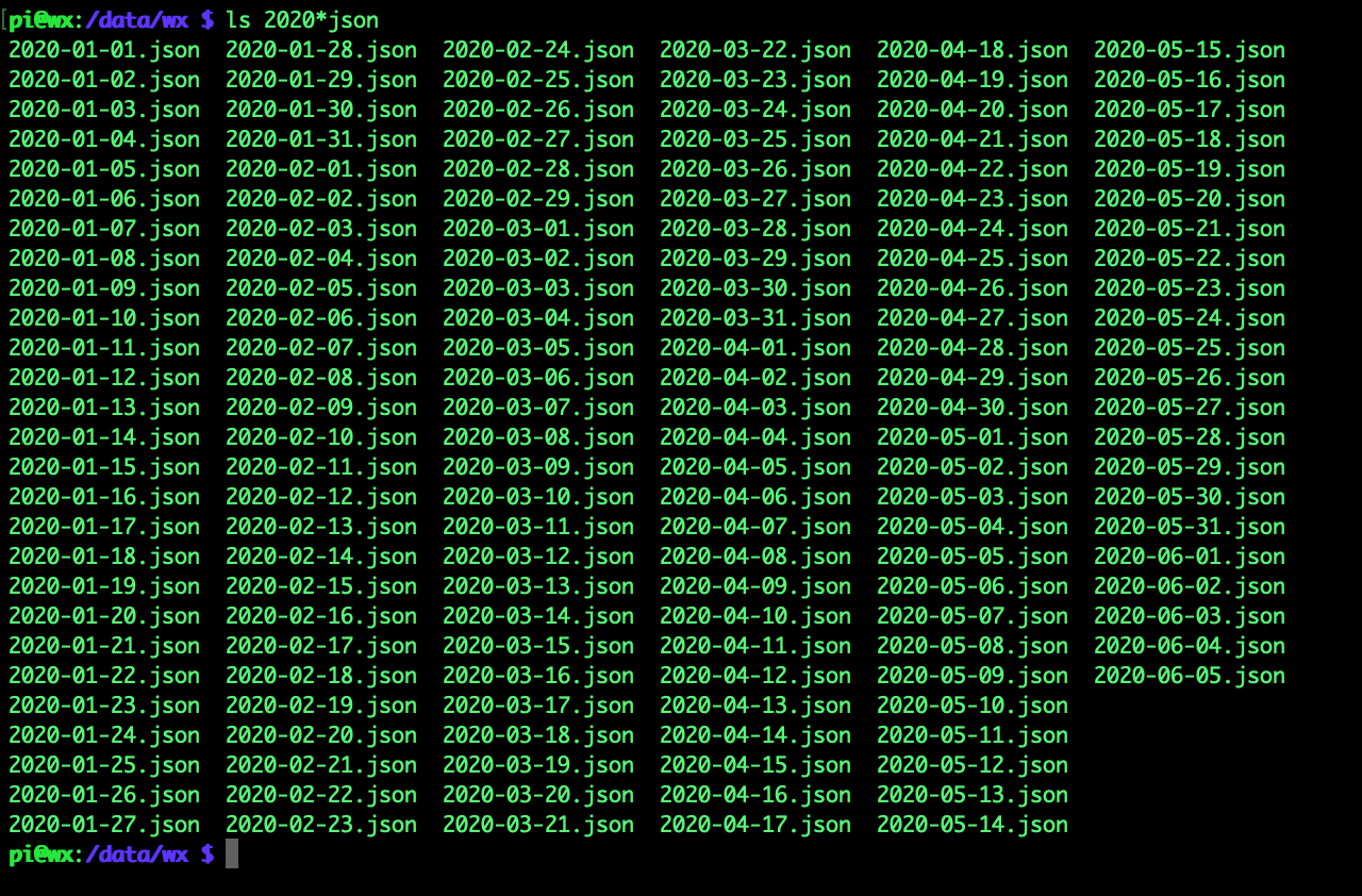
My logger logs to JSON format files by date, which makes it quite easy to munge the data with jq. The folder looks something like this:

Weather Station Datalogger folder listing

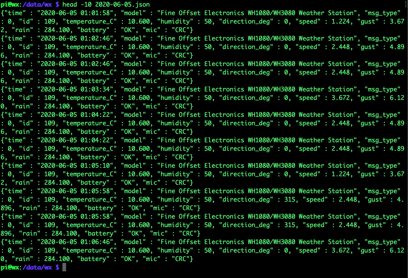
The contents of the files is nicely formatted and mostly looks like this

Weather Station logged data

Meaning I can batter my little raspberry pi and run a bit of jq over all the files:

cat 2020*json | \
jq --slurp 'group_by(.model)|map({model:.[0].model,count:length})'

That is to say: dump all of the 2020 JSON files, slurp them all into a big array in jq, group them into separate arrays by the “model” field, then transform those multiple arrays into just the name from the first element and a count of how many elements were in each array. Neat!

My poor little Pi didn’t like it very much. Each of those files has up to about 3000 records in and slurping the whole lot into memory leads to sad times.

Ok, so running one of the files alone ends up with a clean result

pi@wx:/data/wx $ jq --slurp 'group_by(.model)|map({model:.[0].model,count:length})' 2020-06-05.json
[
 {
  "model": "Ambient Weather F007TH Thermo-Hygrometer",
  "count": 1
 },
 {
  "model": "Citroen",
  "count": 1
 },
 {
  "model": "Elro-DB286A",
  "count": 2
 },
 {
  "model": "Fine Offset Electronics WH1080/WH3080 Weather Station",
  "count": 1956
 },
 {
  "model": "Ford",
  "count": 3
 },
 {
  "model": "Oregon Scientific SL109H",
  "count": 1
 },
 {
  "model": "Renault",
  "count": 3
 },
 {
  "model": "Schrader Electronics EG53MA4",
  "count": 1
 },
 {
  "model": "Smoke detector GS 558",
  "count": 2
 }
]

So mostly weather station data from (presumably!) my WH1080/WH3080 sensor array. The Oregon Scientific SL109H also looks like a weather station – I didn’t think my base station transmitted indoor temps, but I could be mistaken – will have to have a look. Someone else is also running a F007TH Hygrometer doing something similar, too. Citroen, Ford, Renault and Schrader are all tyre pressure sensors of neighbours and/or passing traffic. The Elro-DB286A is a neighbours wireless doorbell… that could be fun spoofing, and the GS558 is obviously a smoke detector, a lot less fun spoofing.

So, I can build tallies for each dated file like so:

for i in 2020*json; do
  cat $i \
  | jq --slurp 'group_by(.model)|map({model:.[0].model,count:length})|.[]';
done > /tmp/2020-tallies.json

Then sum the tallies like so:

cat /tmp/2020-tallies.json | \
jq -s '.|group_by(.model)|map({model:.[0].model,sum:map(.count)|add})'

The data includes a few more devices now, as one might expect. The frequency list looks like this (alphabetical rather than by frequency):

[
 {
  "model": "Acurite 609TXC Sensor",
  "sum": 1
 },
 {
  "model": "Acurite 986 Sensor",
  "sum": 4
 },
 {
  "model": "Akhan 100F14 remote keyless entry",
  "sum": 9
 },
 {
  "model": "Ambient Weather F007TH Thermo-Hygrometer",
  "sum": 13
 },
 {
  "model": "Cardin S466",
  "sum": 12
 },
 {
  "model": "Citroen",
  "sum": 1450
 },
 {
  "model": "Efergy e2 CT",
  "sum": 35
 },
 {
  "model": "Elro-DB286A",
  "sum": 134
 },
 {
  "model": "Fine Offset Electronics WH1080/WH3080 Weather Station",
  "sum": 375066
 },
 {
  "model": "Ford",
  "sum": 4979
 },
 {
  "model": "Ford Car Remote",
  "sum": 31
 },
 {
  "model": "Generic Remote",
  "sum": 28
 },
 {
  "model": "Honda Remote",
  "sum": 55
 },
 {
  "model": "Interlogix",
  "sum": 26
 },
 {
  "model": "LaCrosse TX141-Bv2 sensor",
  "sum": 47
 },
 {
  "model": "Oregon Scientific SL109H",
  "sum": 229
 },
 {
  "model": "Renault",
  "sum": 2334
 },
 {
  "model": "Schrader",
  "sum": 1566
 },
 {
  "model": "Schrader Electronics EG53MA4",
  "sum": 435
 },
 {
  "model": "Smoke detector GS 558",
  "sum": 155
 },
 {
  "model": "Springfield Temperature & Moisture",
  "sum": 2
 },
 {
  "model": "Thermopro TP11 Thermometer",
  "sum": 1
 },
 {
  "model": "Toyota",
  "sum": 474
 },
 {
  "model": "Waveman Switch Transmitter",
  "sum": 2
 }
]

Or like this as CSV:

pi@wx:/data/wx $ cat /tmp/2020-tallies.json | jq -rs '.|group_by(.model)|map({model:.[0].model,sum:map(.count)|add})|.[]|[.model,.sum]|@csv'
"Acurite 609TXC Sensor",1
"Acurite 986 Sensor",4
"Akhan 100F14 remote keyless entry",9
"Ambient Weather F007TH Thermo-Hygrometer",13
"Cardin S466",12
"Citroen",1450
"Efergy e2 CT",35
"Elro-DB286A",134
"Fine Offset Electronics WH1080/WH3080 Weather Station",375066
"Ford",4979
"Ford Car Remote",31
"Generic Remote",28
"Honda Remote",55
"Interlogix",26
"LaCrosse TX141-Bv2 sensor",47
"Oregon Scientific SL109H",229
"Renault",2334
"Schrader",1566
"Schrader Electronics EG53MA4",435
"Smoke detector GS 558",155
"Springfield Temperature & Moisture",2
"Thermopro TP11 Thermometer",1
"Toyota",474
"Waveman Switch Transmitter",2

Removing my weather station from the set, as it dwarfs everything else, the results look like this:

RTL433 Device type frequency in a rural neighbourhood

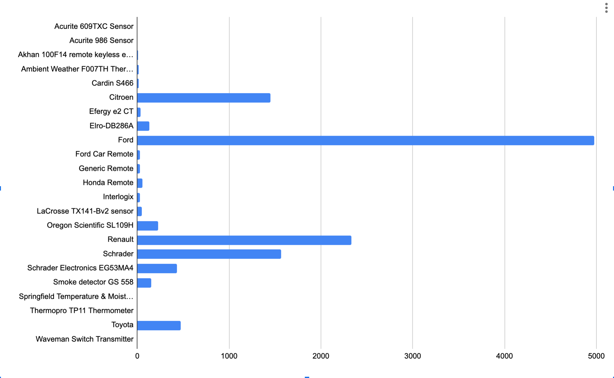
So aside from Ford having the most cars with tyre pressure monitors, it looks like there are a few other interesting devices to explore. Those car remotes don’t feel very secure to me, that’s for sure.

I’ve only just scratched the surface here, so if you’ve found anything interesting yourself with rtl_433, or want me to dig a bit deeper into some of the data I’ve captured here please let me know in the comments.

Bookmarks for March 22nd through August 21st

These are my links for March 22nd through August 21st:

Bookmarks for August 5th through October 14th

These are my links for August 5th through October 14th:

Bookmarks for November 6th through November 26th

These are my links for November 6th through November 26th:

Bookmarks for December 16th through January 11th

These are my links for December 16th through January 11th:

Bookmarks for October 27th through December 7th

These are my links for October 27th through December 7th:

5MHz Propagation Forecasts utilising the Experiment’s Database

Using historical data to predict future conditions

This article, written by Gwyn Williams G4FKH and published in RadCom December 2011 is © RSGB 2011, reproduced with permission.

FIGURE 1: An input form (see text).

BRIEF HISTORY

The RSGB 5MHz Experiment started toward the end of 2002, when the 5MHz Working Group was formed under the chairmanship of John Gould, G3WKL. The current NoVs for access to 5MHz expire on 30 June 2015, but it is possible that Ofcom and MoD will agree to a further extension. The 5MHz Experiment could then run well into the current solar cycle. On the website [1] are various ways in which information can be retrieved from the 5MHz database. In fact there are three separate parts to the database. The first two are concerned with the logging of the three propagation beacons that have been established: the first for manual logging and the second for automated logging. The third part is a compilation of propagation data for the same period. It suddenly occurred to me that the database could be used to forecast propagation.


BASIC CONCEPT

This article and the subsequent web application discuss the automatically logged data and the propagation data. The three beacons in questions are GB3RAL, GB3WES and GB3ORK situated in Maidenhead Locator squares, IO91in, IO84qn and IO89ja respectively. They transmit on a frequency of 5.290MHz every quarter of an hour for one minute each, starting on the hour. Each sequence therefore lasts for three minutes. The logging software was designed by Peter Martinez, G3PLX and is available on the web via the experiment’s main page [1]. To date, the automatic logging part of the database has accumulated over 1.3 million lines of data; the propagation part about one third of this. To perform the forecasts it is necessary to interrogate both of these datasets.
It will be appreciated that there are many stations contributing to the database and therefore there are an equal number of station setups! In order to explain the potential pitfall, I will explain my setup. I have a dipole aerial with a radio and PC. The output from the radio couples to the PC’s soundcard and the program manipulates data from the soundcard. My radio does not provide sufficient output to drive the soundcard, so I have installed an inline amplifier. I can, therefore, adjust my own recorded background/signal strength. Not taking care when analysing the data will cause these differences to become exaggerated. The G3PLX program compensates somewhat for this internally and displays the background signal level and the SNR of the station being monitored. This internal rationalisation and the forecasting program’s own scheme mitigate these differences.

I write small computer programs in the Perl language; during a fairly recent local club meeting I discussed this idea with Roger Pettett, G7TKI, a professional systems developer. My personal experience is not up to his standard and, as Roger kindly volunteered to develop the program in his own time, I quickly agreed. Roger is not au fait with propagation so the collaboration is a good one.


5MHz PROPAGATION

Before I go on to discuss the developed program and its usage, it seems expedient to first outline propagation at this frequency. Most of the propagation at this QRG is via NVIS (near vertical incidence skywave) communication. The E-layer (and probably, during some periods, the F-layer) do influence the longer distance circuits. NVIS for most practical purposes has a range of about 400km; therefore, if a station is set up in the middle of the UK, NVIS would be the dominant mode for the whole of the country. However, we do not live in an idealised world so a method is needed to perform forecasts between any two parts of the UK. To facilitate this database locators are used to correlate distances. The R12 (twelve-month smoothed relative sunspot number) and the AP (planetary A-index) are used to represent propagation conditions. R12 is automatically retrieved from the internet, but it is necessary to input the AP [2] that represents the propagation conditions under consideration. The best results within the UK will be achieved when using a 1⁄2λ dipole; the program suggests some aerial dimensions.
The ionosphere is fed by ionisation from the sun and this has a direct correlation with sunspot numbers. The ionosphere requires X amount of ionisation to allow for NVIS communication. For simplicity we can view the AP as a measure of disturbance in the ionosphere. The higher the AP, the worse the propagation will become.

Instead of using propagation prediction engines, eg VOACAP, we interrogate the databases to find parity (within parameters) to those conditions input by the user. A more complete introduction to NVIS communications can be found in [3].

5MHz FORECASTING PROGRAM

The completed program can be found at [4] and should be straightforward in use. As mentioned it is only necessary to input the AP, month, year and locator squares that are to be forecast, the last input tick is for a smoothed graph output. Figure 1 is an example of the input form. It can take a little time to search through the databases to find the correct matches; when the relevant data are found a table like Table 1 is produced along with a graph, Figure 2.

The table, which can be viewed as a median for a whole month, comprises three headed columns. The first column is the hour of the day, the second an SNR (signal to noise ratio) for the hour and the third an explanatory note for the SNR. For the purposes of this dataset an SNR below 20 should be considered as unreadable. The graph is a pictorial view of the table data; the thin green line is where the signal drops out of usability.
It may not be apparent why we need a tool such as the one described, because after all we have experience at this QRG and have other prediction tools at our left hand. What these things do not provide is the ability to visualise propagation when conditions are disturbed or changing. Inputting the correct answers into the input form allows the user to see what conditions will be like when the ionosphere becomes disturbed, such as from Coronal Mass Ejections and solar flares. This ability is lacking in prediction engines, but this program shows to what extent any degree of disturbance should have upon any circuit. However, there is one short-coming suffered by all forecasting tools and that is the ability to see things before they happen, ie a short- wave-fade from a large flare. This effect will last the same amount of time as the flare is visible from Earth (utilising the correct viewing techniques), from a minute or two, to perhaps an hour or so. These effects have a quick onset and an equally quick fall-off period.
Comparatively speaking and from interest the output from this program was compared with REC533, the same prediction engine used to produce the RadCom predictions (to be fair, predictions programs were never really designed for such short distances).
A survey was produced for RadCom in 2000 and REC533 was found to perform best. Comparing the output from REC533 (Table 2 Predicted SNR column) and what was actually copied using the automatic monitoring program (Table 2 Automatic Recording SNR column) showed that REC533 was only 25% accurate. When it is considered that this percentage of accuracy is only obtainable when geomagnetic conditions are quiet it shows a severe shortcoming.

Comparing this to the output from our new program (Table 2 Forecast SNR column) with an accuracy of 67% against actual monitoring, under all geomagnetic conditions, it shows the new program to be far superior to anything previously available. Comparison was carried out with the criteria of the SNR being within 10dB. In order to obtain more accurate results more data is required as well as data from a greater number of stations.
Table 3 and Figure 3 demonstrate the way in which conditions can change in reality. These clearly demonstrate the different conditions when an ionospheric disturbance is at hand. Of course it should be understood that diurnal conditions also have a bearing on the results shown in the table, ie at the very end and very beginning of the day, for some circuits no path is expected. What is happening is that the foF2 (F2 critical frequency) is dropping below the required frequency; this is when the E and F layers can accommodate communication.


SUMMARY

This simple but effective idea can prove useful in all sorts of circumstances, ie for everyday amateur use, emergency situations (RAYNET) and other occasions outside the amateur service where 5MHz is in use, especially when conditions become disturbed during ionospheric upheavals. It is the use of a database with all varieties of propagation conditions that is the winning ingredient in performing accurate forecasts. As the database builds up to a crescendo in 2015, a whole solar cycle and more of information will have been logged and will provide an unsurpassed amount of quality data for this frequency.


WEBSEARCH

[1] www.rsgb.org/spectrumforum/hf/5mhz.php
[2] www.swpc.noaa.gov/ftpdir/weekly/27DO.txt
[3] Near Vertical Incidence Skywave Communication, Theory, Techniques and Validation by LTC, David M Fiedler, (NJ ARNG) (Ret) and MAJ Edward J Farmer, PE (CA SMR). Published by Worldradio Books,
[4] www.rsgb-spectrumforum.org.uk/5mhzpf

This article may also be downloaded in PDF format here: 5MHz Propagation Forecasting utilising the Experiment’s Database

Bookmarks for July 20th through September 15th

These are my links for July 20th through September 15th:

Bookmarks for June 10th through June 27th

These are my links for June 10th through June 27th:

Bookmarks for April 28th through May 15th

These are my links for April 28th through May 15th: